
Forecasting US Honey Production and Price
Overview
My previous two posts explored US honey production and identified key relationships between the supply of honey and its price. In this post, I will build on insights gained there to develop models that will allow me to make predictions about the future US honey market. In particular, I want to determine: How much honey will be on the domestic market at some time in the future? What will be the price of honey at that time?
Based on what I learned in my previous projects, the answer to the second question depends on the answer to the first. So, I will need to build two predictive models: one model to forecast the future market size of honey in each state and another model to predict, based on the results of the first model, the future price of that honey.
The future market size of honey can be forecasted with a time-series model. Time-series models assess both long term and short term trends over the timespan of the dataset to predict future events. Since each state is independent, the market size of each state will need to be modeled separately. Therefore, the first model I will build is an ensemble of time-series models for each state where I determined the optimal forecasting method to predict the amount of honey that state will produce in subsequent years.
Next, the price of honey will be modeled using machine learning regression algortihms. Feeding the results of the market size forecast into this model, I can predict the price of honey in the future.
This blog post contains the broad brush description of the construction of these two models. Additional details and the code used to make the figures can be found in the accompanying notebook.
About the data
The honey market dataset used in part 1 and 2 covered the years 1999-2012. Wanting this project to be more current, I downloaded the raw data for US honey production for 2013-2017 from the US Department of Agriculture. I cleaned and processed the data to match the format of the earlier dataset and the notebook containing that procedure can be found here.
Combining the data together, I have a lot of latitude in terms of how to build a predictive model. Ultimately, the model I will build could be used to predict this year’s production and price, however then I would need to wait to see if I was correct (and that is no fun). So, I chose instead to make a multiyear prediction for 2015-2017 so I can compare the model predictions with the actual supply of honey on the US market. This is a little like pretending I am data scientist in 2014 and predicting the price for the next 3 years.
California market size forecast
The first goal is to build a time series model to predict the market size of each state for 2015-2017 based on the data from 1999-2014. In order to develop some intuition on how best to do this, I examined several forecasting methods for the market size on a singe state, California, in detail. California is one of the larger honey producing states, so it is great sandbox for experimentation.
In order to evaluate the effectiveness of the modelling process, I needed to divide the California dataset into a training and testing set. I settled on a training set of the California honey market size for 1999-2011 which I used to build a model and make a multiyear prediction for 2012-2015. Then, I evaluated the accuracy of those predictions by comparing against the testing dataset of the acutal California honey market size values for 2012-2015.
I considered three time-series models (in order of increasing complexity): a) a linear trend model, b) a moving average model, and c) a Holt-Winters seasonal model. Detailed descriptions of each of these models can easily be found elsewhere, but I briefly summarize them as follows: A linear trend model simply fits a fixed linear trend to the data. The moving average model predicts the i-th point by averaging that step with the previous N-1 steps, where N is a tunable parameter that is determined through an optimization routine. Lastly, the Holt-Winters model uses an exponential weighted moving average and adds a seasonal variation to respectively model long and short term trends in the data.
I did some experimenting with a seasonal Autoregressive Integrated Moving Average (SARIMA) model, which is a popular choice in time-series modeling. But given the relative small sample of data points, I decided that it was too complex for this dataset.
The results of the three models for California are shown below.
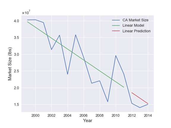
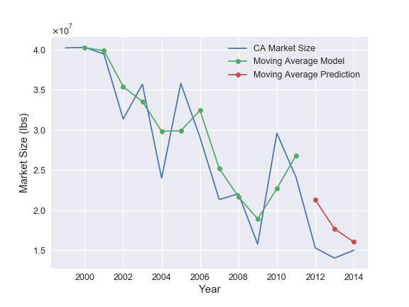
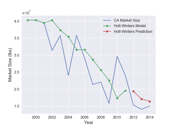
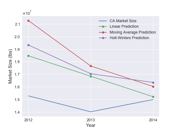
The figures show that there is a parameterization for each of the three time-series models that can reasonably represent the data and make competitive predictions. For California, the linear trend model makes slightly more accurate predictions than the other two. Therefore, these are the model results that would be selected by the pipeline that is discussed in the next section.
It is possible that a different time-series model that I am not considering here could do a better job than the three I have chosen. However, given the limited size of the dataset, these are reasonable enough results that I can proceed to the next step and leave consideration of other time-series models for another time (if necessary).
Forecast pipeline for all states
After confirming that these models are competitive in forecasting the production of one state, I built a pipeline that identifies the best method for each state and forecasts that state’s market size for 2015-2017. For example, in the case of Alabama, the Holt-Winters model (parameterized with a seasonal_period = 3) is the optimal model and is expected to provide the most accurate forecast of Alabama’s future market size.
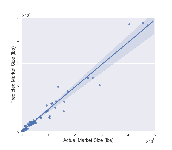
According to the plot below the ensemble model does a good job predicting future honey market sizes for each state. There is a nearly one-to-one relationship between predicted and actual market size values and the residuals (see accompanying notebook) have an approximately normal distribution. If I wanted to improve this model further I could look to do a better job with the larger markets, however for the purposes of answering the main questions of this blog entry, these results are sufficient.
Predicting the price of honey with Machine Learning
Now that I have a forecast for the future market size of honey in each state, I can construct a model to use that information to predict the future price. To do that I am going to utilize machine learning regression algorithms. There are a wealth of regression models, but after some exploration I settled on a Random Forest regression model. The full model fitting and evaluation process is described in the notebook.
Random Forests are an ensemble method that utilize a collection of Decision Trees built from subsamples of the dataset. A Decision Tree is a machine learning algorithm that makes a series of decisions on how to informatively divide the training data in order to predict the target feature. Random Forests make accurate predictions by aggregating the results of a large number of individual trees. This method excels in identifying non-linear relationships and is robust against overfitting due to its internal calculation of error during training. This makes Random Forest regression an ideal choice for the problem at hand.
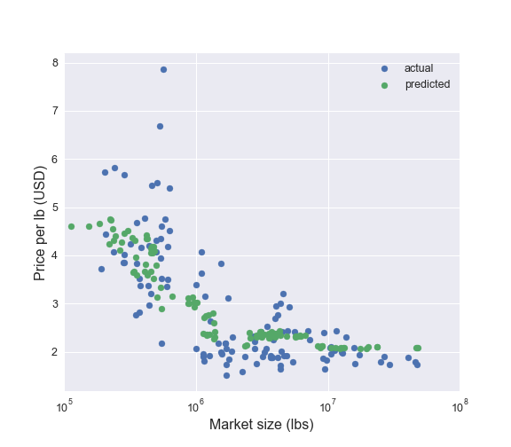
The plot below illustrates how well Random Forest regression does predicting the price of honey for each state from the forecasted market size from 2015-2017. The overall trend in the predicted price with respect to the market size matches up well with the actual values. However, there is some scatter in the real data that the model is unable to account for. In terms of predicting individual state prices this model may be able to be improved upon, but it describes the aggregate US market and pricing well.
Finally, I can use this model to answer the original motivating questions: How much honey will be on the domestic market at some time in the future? What will be the price of honey at that time?
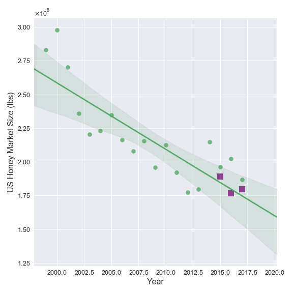
The predictions for the total US market size and the mean price for 2015-2017 are shown in the figures below as purple squares. The actual dataset values for 1999-2017 are also shown and fit with linear trends (as in my first blog post). The figures clearly show that the predicted domestic market size and the mean US price are pretty close to the actual values. Two of the three predicted prices are nearly exact matches with the real data!
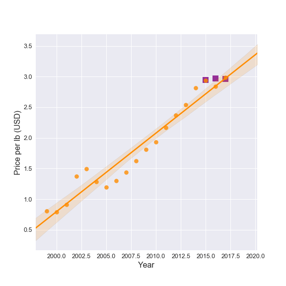
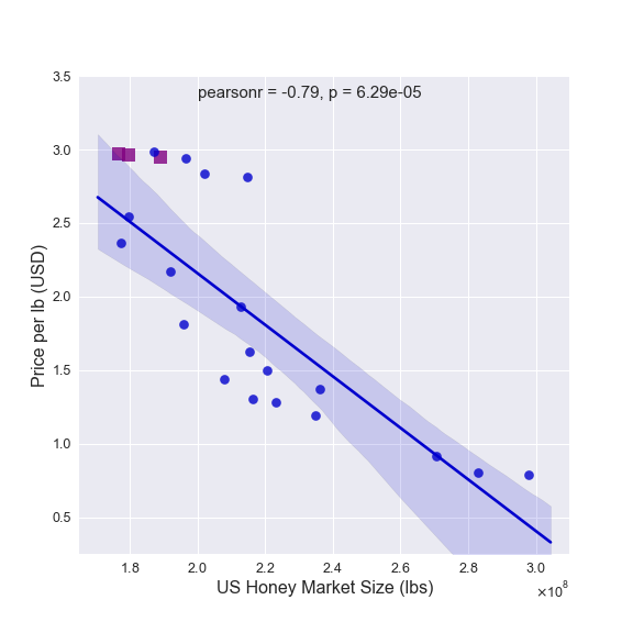
The figure above also indicates how this entire modelling process can be improved upon. The predicted price for 2016 is the most divergent from the actual value where the market size prediction also has the largest offset. This implies that improving the forecasting model for domestic market size will reduce the error in the price prediction. As stated above, the larger errors in the market size forecasting model came from the states with the bigger market sizes, thus having the largest impact on the prediction of the total US market. Any future improvements to this modelling procedure should focus on producing a better market size forecast for the small number of states with larger markets that were identified in the previous blog post.
Summary
The future amount of honey on the market in each state for 2015-2017 was forecasted using an ensemble of time-series models where the optimal algorithm was selected individually for each state. The price of that honey was predicted utilizing supervised learning of a Random Forest regression model. In terms of forecasting for individual states there are places where the models can do better, namely: improved market size forecasting for states with larger markets. All considered, for a 3 year projection with a relatively small dataset, this aggregate model does a very good job at predicting both the total domestic market size of and the mean price of honey.